Chapter 3 Writing R Code

3.1 Writing Style

When writing code it is important to follow a common style so it is readable and other people, and your future self, can easily understand and extend it.

3.1.1 Tidyverse

It is recommended, when using R, that we use the “Tidyverse” approach and packages wherever possible. The Tidyverse is a collection of packages designed for data science, as well as a philosophy and style for formatting data and writing functions. The tidyverse.org website details the packages involved and contains articles on how to use them. Some of it will be summarised below, but the website contains the definitive information.

The most in-depth treatment on the Tidyverse can be found in the book R for Data Science, which is available online for free at r4ds.had.co.nz.

The tidyverse has an extensive style guide, which we summarise here:

3.1.2 Files

File names should be meaningful and end in .R, or .Rmd for R markdown files. Only use letters, numbers and - or _.
If your script required packages load them all at once at the very beginning of the file.
Use comments to explain the “why” not the “what” or “how”.
Break up files into named sections using commented lines (# ----, example below). In RStudio you can collapse and expand sections commented this way.

# Load data --------------------------------------------------------------------

3.1.3 Syntax

Variable and function names should use only lowercase letters, numbers, and _.
Always indent the code inside curly braces {} by two spaces.

3.1.4 Functions

Use verbs for function names where possible.
If a function has numerous arguments put each one on a new line.
A function should do one thing well. If it is doing too much the break it up.
A function should be easily understandable in isolation. It should not refer to any variables outside the function scope.

3.1.5 Pipes

Use %>% when you find yourself composing three or more functions together, instead of a nested call.
%>% should always have a space before it and a new line after it. After the first step, each line should be indented by two spaces.

3.1.6 Documentation

Created functions should be documentated so others, including the future you, can understand what the function does and how to use it.
Documentation should be written before the function definition in an roxygen2 style. roxygen uses special comments, starting with #'. The first line is the title, and anything else, not prefixed with a keyword forms the description. Keywords start with @ and the most important ones are @param to describe a function parameter and @return to describe what the function returns.

Here is a very simple example:

#' The length of a string.
#'
#' This function returns the number of characters in the supplied string.
#' 
#' @param string input character vector
#'
#' @return integer vector giving number of characters in each element of the
#'   character vector.
#'
#' @export
#'
str_length <- function(string) {
  nchar(string)
}

3.2 Structure

Organising files for a particular piece of work becomes more important as the scale and complexity increases. Standard approaches exists to simplify the workflow.

3.2.1 Projects

Use RStudio projects to organise files. This has a number of advantages:

Sets the working directory to the project location
Reopens the same files when returning to the projects
Saves the workspace so data and code is loaded when you re-open the project

3.2.2 Folders

When an analysis becomes complex it should be split up into logical parts and stored in subfolders. Store the original data in a folder, unchanged. It is better to “cleanse” input data with an R script as it can repeated when data changes, and/or the approach changed itself.

R code may also be stored in a separate folder. You may have an R script for cleansing the data and another for performing an analysis. Include an R script at the top level which executes the code in the subfolder in the appropriate order. Use relative paths to the files. If an RStudio project has been created the working directory will be set to the project directory automatically.

Output the results, plots, data, etc, in another folder so it is clear whether data files are results rather than inputs.

An example of a project structure:

data
- interesting-data.xlsx
- reference-data.csv
R
- clean-data.R
- analyse.R
tests
- test-cleansed-data.R
- test-analysis.R
results
- cool-plot.png
- table-of-results.csv
run-code.R
README.md

3.2.3 README

Adding a README file is a good way to explain to other, and you future self, what the analysis does and how to use it. The documentation section of the best practice has more detail on what should be included.

It is recommended that markdown is used to write the README. It is a very simple way to specify text formatting in a plain text file and can be converted to many other formats (HTML, docx, PDF) if required. In addition, if the package is stored in GitHub a markdown README is automatically rendered on the repository’s page.

3.2.4 R Packages

When R code has high criticality consider turning it into a package. A package is a way of collecting together related code in a robust way. It has the following advantages:

Easier to share with others (as a zip file)
Documentation is compiled into help pages
All tests can be executed with a single command
Can implement a development and release process
Code is broken up into useful functions

Writing a package is very straight forward with the helper packages available today. More information can be found in Package Development.

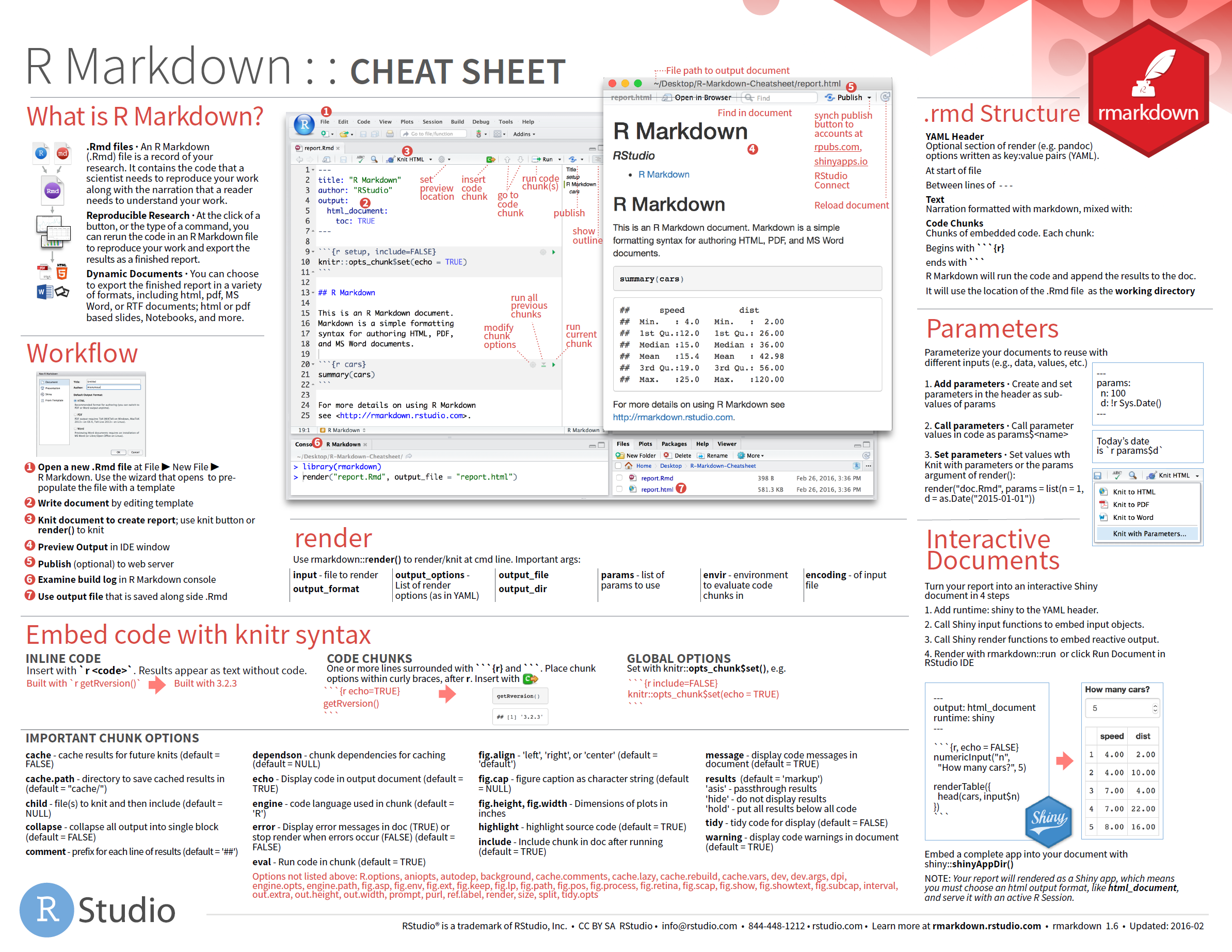
3.3 R Markdown

R markdown is a way of capturing documentation, code and results and in a single file. The document is written in plain text using a style called markdown. This has a simple syntax for specifying text formatting. R code is added in “chunks” and when the document is rendered the R code is executed and replaced with the results.

R markdown can be used to produce web pages, Word and PDF documents. The provide a robust way of capturing an analysis and the results and can be re-run when the data changes.

RStudio provides a cheatsheet detailing R markdown functionality:

For a detailed guide the book R Markdown is available for free online.

3.3.1 Markdown

Markdown is a lightweight markup language with plain text formatting syntax. It is designed so that it can be converted to HTML and many other formats.

3.3.1.1 Paragraphs

Leave at least one empty line between text to start a new paragraph.

This is the first paragraph.

This is the second paragraph.

This is the first paragraph.

This is the second paragraph.

3.3.1.2 Headers

# Header 1

## Header 2

### Header 3

3.3.1.3 Emphasis

*italic*   **bold**

_italic_   __bold__

italic bold

3.3.1.4 Lists

Unordered List:

* Item 1
* Item 2
    + Item 2a
    + Item 2b

Item 1
Item 2
- Item 2a
- Item 2b

Ordered List:

1. Item 1
2. Item 2
3. Item 3
    a. Item 3a
    b. Item 3b

Item 1
Item 2
Item 3
1. Item 3a
2. Item 3b

3.3.1.5 Links

Use a plain http address or add a link to a phrase:

http://example.com

[linked phrase](http://example.com)

http://example.com

linked phrase

3.3.1.6 Images

Images on the web or local files in the same directory:

![](https://upload.wikimedia.org/wikipedia/commons/1/1b/R_logo.svg)

![optional caption text](images/octocat.png)

optional caption text

3.3.1.7 Reference Style Links and Images

Links

A [linked phrase][id].

At the bottom of the document:

[id]: http://example.com/ "Title"

A linked phrase.

At the bottom of the document:

Images

![alt text][id]

At the bottom of the document:

[id]: images/octocat.png "Octocat"

alt text

At the bottom of the document:

3.3.1.8 Blockquotes

A friend once said:

> It's always better to give
> than to receive.

A friend once said:

It’s always better to give than to receive.

3.3.1.9 Plain Code Blocks

Plain code blocks are displayed in a fixed-width font but not evaulated

```
This text is displayed verbatim / preformatted
```

This text is displayed verbatim / preformatted

3.3.1.10 Inline Code

We defined the `add` function to compute the sum of two numbers.

We defined the add function to compute the sum of two numbers.

3.3.1.11 LaTeX Equations

Inline equation:

Einstein's famous equation $E = mc^2$

Einstein’s famous equation \(E = mc^2\)

Display equation:

$$
E = mc^2
$$

\[ E = mc^2 \]

3.3.1.12 Horizontal Rule / Page Break

Three or more asterisks or dashes:

******

------

3.3.1.13 Tables

First Header  | Second Header
------------- | -------------
Content Cell  | Content Cell
Content Cell  | Content Cell

First Header	Second Header
Content Cell	Content Cell
Content Cell	Content Cell

3.3.1.14 Manual Line Breaks

End a line with a backslash:

Roses are red,\
Violets are blue.

Roses are red,
Violets are blue.

3.3.1.15 Miscellaneous

superscript^2^

~~strikethrough~~

superscript²

~~strikethrough~~

3.3.2 R Code Chunks

R code surrounded with three ticks and designated {R} (see below) will be evaluated and printed.


```r
summary(cars$dist)

##    Min. 1st Qu.  Median    Mean 3rd Qu.    Max. 
##    2.00   26.00   36.00   42.98   56.00  120.00

summary(cars$speed)

##    Min. 1st Qu.  Median    Mean 3rd Qu.    Max. 
##     4.0    12.0    15.0    15.4    19.0    25.0



```r
summary(cars$dist)

##    Min. 1st Qu.  Median    Mean 3rd Qu.    Max. 
##    2.00   26.00   36.00   42.98   56.00  120.00

summary(cars$speed)

##    Min. 1st Qu.  Median    Mean 3rd Qu.    Max. 
##     4.0    12.0    15.0    15.4    19.0    25.0

Inline R Code:

There were 50 cars studied

There were 50 cars studied

There are many options available when executing R code chunks. For more information read the R code chunks chapter in the R Markdown book.

3.3.3 R Notebooks

An R Notebook is an R Markdown document with chunks that can be executed independently and interactively, with output visible immediately beneath the input. They direct interaction with R while producing a reproducible document with publication-quality output.

Any R Markdown document can be used as a notebook, and all R Notebooks can be rendered to other R Markdown document types. A notebook can therefore be thought of as a special execution mode for R Markdown documents. The immediacy of notebook mode makes it a good choice while authoring the R Markdown document and iterating on code. When you are ready to publish the document, you can share the notebook directly, or render it to a publication format with the Knit button.

3.3.3.1 Creating a Notebook

You can create a new notebook in RStudio with the menu command File -> New File -> R Notebook, or by using the html_notebook output type in your document’s YAML metadata.

---
title: "My Notebook"
output: html_notebook
---

3.3.3.2 Inserting chunks

Notebook chunks can be inserted quickly using the keyboard shortcut Ctrl + Alt + I, or via the Insert menu in the editor toolbar.

Because all of a chunk’s output appears beneath the chunk (not alongside the statement which emitted the output, as it does in the rendered R Markdown output), it is often helpful to split chunks that produce multiple outputs into two or more chunks which each produce only one output.

3.3.4 Executing chunks

To execute a chunk of code use the green triangle button on the toolbar of a code chunk that has the tooltip “Run Current Chunk”, or Ctrl + Shift + Enter to run the current chunk. The result is then displayed underneath the chunk.